Deep Active Learning with Frozen Vision Transformer#
Google Colab Note: If the notebook fails to run after installing the needed packages, try to restart the runtime (Ctrl + M) under Runtime -> Restart session.
![]()
Notebook Dependencies
Uncomment the following cells to install all dependencies for this tutorial.
[ ]:
# !pip install scikit-activeml[opt] torch torchvision tqdm datasets transformers
This tutorial aims to demonstrate a practical comparison study using our scikit-activeml library. The workflow involves utilizing a self-supervised learning model, specifically DINOv2 from [1], to generate embeddings for the CIFAR-100 dataset [2]. Subsequently, various active learning strategies will be employed to intelligently select samples for labeling.
Key Steps:
Self-Supervised Learning Model: Utilize the DINOv2 model to create embedding dataset for CIFAR-100 dataset.
Active Learning Strategies: Employ different active learning strategies provided by our library, including:
Random Sampling,
Uncertainty Sampling,
Discriminative Active Learning,
CoreSet,
TypiClust,
Badge,
ProbCover,
DropQuery,
Falcun.
Batch Sample Selection: Use each active learning strategy to select a batch of samples for labeling.
Plotting the results: By the end of this notebook, we’ll compare the accuracy of the aforementioned active learning strategies.
References:
[1] Oquab, M., Darcet, T., Moutakanni, T., Vo, H. V., Szafraniec, M., Khalidov, V., … & Bojanowski, P. DINOv2: Learning Robust Visual Features without Supervision. Transactions on Machine Learning Research.
[2] Krizhevsky, A., & Hinton, G. (2009). Learning Multiple Layers of Features from Tiny Images.
[2]:
# Comment in for speedup, if you have cuML installed.
# %load_ext cuml.accel
import numpy as np
import matplotlib as mlp
import matplotlib.pyplot as plt
import torch
import warnings

from datasets import load_dataset
from sklearn.linear_model import LogisticRegression
from skactiveml.classifier import SklearnClassifier
from skactiveml.pool import (
    UncertaintySampling,
    RandomSampling,
    DiscriminativeAL,
    CoreSet,
    TypiClust,
    Badge,
    DropQuery,
    ProbCover,
    Falcun,
    SubSamplingWrapper,
)
from skactiveml.utils import call_func
from transformers import AutoImageProcessor, Dinov2Model
from tqdm import tqdm


warnings.filterwarnings("ignore")
mlp.rcParams["figure.facecolor"] = "white"
device = "cuda" if torch.cuda.is_available() else "cpu"
cuML: Accelerator installed.
Embed CIFAR-100 Images with DINOv2#
In this step, we focus on preparing the datasets using the self-supervised learning model DINOv2. DINOv2, short for “self-distillation with no labels”, is a popular vision foundation model that excels at providing meaningful representations for image data.
[3]:
# Download data.
ds = load_dataset("uoft-cs/cifar100")

# Download DINOv2 ViT/S-14 as embedding model.
processor = AutoImageProcessor.from_pretrained(
    "facebook/dinov2-small", use_fast=True
)
model = Dinov2Model.from_pretrained("facebook/dinov2-small").to(device).eval()


# Embed CIFAR-100 images.
def embed(batch):
    inputs = processor(images=batch["img"], return_tensors="pt").to(device)
    with torch.no_grad():
        out = model(**inputs).last_hidden_state[:, 0]
    batch["emb"] = out.cpu().numpy()
    return batch


ds = ds.map(embed, batched=True, batch_size=32)
X_pool = np.stack(ds["train"]["emb"], dtype=np.float32)
y_pool = np.array(ds["train"]["fine_label"], dtype=np.int64)
X_test = np.stack(ds["test"]["emb"], dtype=np.float32)
y_test = np.array(ds["test"]["fine_label"], dtype=np.int64)
Random Seed Management#
To ensure experiment reproducibility, it’s important to set random states for all components that might use them. For simplicity, we set a single fixed random state and use helper functions to generate new seeds and random states. It’s important to note that the master_random_state should only be used to create new random states or random seeds.
[4]:
master_random_state = np.random.RandomState(0)


def gen_seed(random_state: np.random.RandomState):
    """
    Generate a seed for a random number generator.

    Parameters:
    - random_state (np.random.RandomState): Random state object.

    Returns:
    - int: Generated seed.
    """
    return random_state.randint(0, 2**31)


def gen_random_state(random_state: np.random.RandomState):
    """
    Generate a new random state object based on a given random state.

    Parameters:
    - random_state (np.random.RandomState): Random state object.

    Returns:
    - np.random.RandomState: New random state object.
    """
    return np.random.RandomState(gen_seed(random_state))
Classification Models and Query Strategies#
The embeddings we have computed can be used as an input to a classification model. For this guide, we use LogisticRegression from sklearn. Moreover, we handle the creation of query strategies using factory functions to simplify the separation of query strategies across repetitions.
[5]:
n_features, classes = X_pool.shape[1], np.unique(y_pool)
missing_label = -1
clf = SklearnClassifier(
    LogisticRegression(verbose=0, tol=1e-3, C=0.01, max_iter=10000),
    classes=classes,
    random_state=gen_seed(master_random_state),
    missing_label=-1,
)


def create_query_strategy(name, random_state):
    return query_strategy_factory_functions[name](random_state)


query_strategy_factory_functions = {
    "RandomSampling": lambda random_state: RandomSampling(
        random_state=gen_seed(random_state), missing_label=missing_label
    ),
    "UncertaintySampling": lambda random_state: UncertaintySampling(
        random_state=gen_seed(random_state), missing_label=missing_label
    ),
    "DiscriminativeAL": lambda random_state: DiscriminativeAL(
        random_state=gen_seed(random_state), missing_label=missing_label
    ),
    "CoreSet": lambda random_state: CoreSet(
        random_state=gen_seed(random_state), missing_label=missing_label
    ),
    "TypiClust": lambda random_state: TypiClust(
        random_state=gen_seed(random_state), missing_label=missing_label
    ),
    "Badge": lambda random_state: Badge(
        random_state=gen_seed(random_state), missing_label=missing_label
    ),
    "DropQuery": lambda random_state: DropQuery(
        random_state=gen_seed(random_state),
        missing_label=missing_label,
    ),
    "ProbCover": lambda random_state: ProbCover(
        random_state=gen_seed(random_state), missing_label=missing_label
    ),
    "Falcun": lambda random_state: Falcun(
        random_state=gen_seed(random_state), missing_label=missing_label
    ),
}
Experiment Parameters#
For this experiment, we need to define how the strategies should be compared against one another. Here the number of repetitions (n_reps), the number of cycles (n_cycles), and the size of each query (query_batch_size) need to be defined.
[6]:
n_reps = 3
n_cycles = 20
query_batch_size = 100
query_strategy_names = query_strategy_factory_functions.keys()
Experiment Loop#
The actual experiment loops over all query strategies. The accuracy for the test set is stored for each cycle and repetition in the results dictionary.
[7]:
results = {}
for qs_name in query_strategy_names:
    accuracies = np.full((n_reps, n_cycles + 1), np.nan)
    for i_rep in range(n_reps):
        y_train = np.full(shape=len(X_pool), fill_value=missing_label)

        qs = create_query_strategy(
            qs_name,
            random_state=gen_random_state(np.random.RandomState(i_rep)),
        )
        qs = SubSamplingWrapper(
            query_strategy=qs,
            missing_label=missing_label,
            random_state=gen_random_state(np.random.RandomState(i_rep)),
            exclude_non_subsample=True,
            max_candidates=0.1,
        )
        clf.fit(X_pool, y_train)
        accuracies[i_rep, 0] = clf.score(X_test, y_test)

        for c in tqdm(
            range(1, n_cycles + 1), desc=f"Repeat {i_rep + 1} with {qs_name}"
        ):
            query_idx = call_func(
                qs.query,
                X=X_pool,
                y=y_train,
                batch_size=query_batch_size,
                clf=clf,
                discriminator=clf,
                update=True,
            )
            y_train[query_idx] = y_pool[query_idx]
            clf.fit(X_pool, y_train)
            accuracies[i_rep, c] = clf.score(X_test, y_test)

    results[qs_name] = accuracies
Repeat 1 with RandomSampling: 100%|██████████| 20/20 [00:00<00:00, 23.92it/s]
Repeat 2 with RandomSampling: 100%|██████████| 20/20 [00:00<00:00, 27.29it/s]
Repeat 3 with RandomSampling: 100%|██████████| 20/20 [00:00<00:00, 27.51it/s]
Repeat 1 with UncertaintySampling: 100%|██████████| 20/20 [00:01<00:00, 16.92it/s]
Repeat 2 with UncertaintySampling: 100%|██████████| 20/20 [00:01<00:00, 17.31it/s]
Repeat 3 with UncertaintySampling: 100%|██████████| 20/20 [00:01<00:00, 17.56it/s]
Repeat 1 with DiscriminativeAL: 100%|██████████| 20/20 [01:09<00:00,  3.48s/it]
Repeat 2 with DiscriminativeAL: 100%|██████████| 20/20 [01:09<00:00,  3.47s/it]
Repeat 3 with DiscriminativeAL: 100%|██████████| 20/20 [01:10<00:00,  3.53s/it]
Repeat 1 with CoreSet: 100%|██████████| 20/20 [00:05<00:00,  3.82it/s]
Repeat 2 with CoreSet: 100%|██████████| 20/20 [00:05<00:00,  3.86it/s]
Repeat 3 with CoreSet: 100%|██████████| 20/20 [00:05<00:00,  3.78it/s]
Repeat 1 with TypiClust: 100%|██████████| 20/20 [00:09<00:00,  2.19it/s]
Repeat 2 with TypiClust: 100%|██████████| 20/20 [00:09<00:00,  2.20it/s]
Repeat 3 with TypiClust: 100%|██████████| 20/20 [00:09<00:00,  2.19it/s]
Repeat 1 with Badge: 100%|██████████| 20/20 [04:07<00:00, 12.36s/it]
Repeat 2 with Badge: 100%|██████████| 20/20 [04:09<00:00, 12.47s/it]
Repeat 3 with Badge: 100%|██████████| 20/20 [04:07<00:00, 12.40s/it]
Repeat 1 with DropQuery: 100%|██████████| 20/20 [00:04<00:00,  4.07it/s]
Repeat 2 with DropQuery: 100%|██████████| 20/20 [00:04<00:00,  4.10it/s]
Repeat 3 with DropQuery: 100%|██████████| 20/20 [00:04<00:00,  4.14it/s]
Repeat 1 with ProbCover: 100%|██████████| 20/20 [00:24<00:00,  1.24s/it]
Repeat 2 with ProbCover: 100%|██████████| 20/20 [00:24<00:00,  1.24s/it]
Repeat 3 with ProbCover: 100%|██████████| 20/20 [00:24<00:00,  1.24s/it]
Repeat 1 with Falcun: 100%|██████████| 20/20 [00:01<00:00, 10.46it/s]
Repeat 2 with Falcun: 100%|██████████| 20/20 [00:01<00:00, 10.24it/s]
Repeat 3 with Falcun: 100%|██████████| 20/20 [00:01<00:00, 10.32it/s]
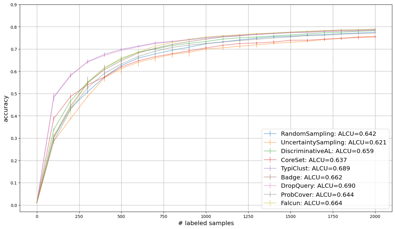
Resulting Plotting#
We use learning curves to compare strategies. We visualize the average accuracy over all repetitions. In addition, the legend provides insight into the area under the learning curve, which indicates the average accuracy over all cycles.
[8]:
plt.figure(figsize=(16, 9))
for qs_name in query_strategy_names:
    key = qs_name
    result = results[key]
    reshaped_result = result.reshape((-1, n_cycles + 1))
    errorbar_mean = np.mean(reshaped_result, axis=0)
    errorbar_std = np.std(reshaped_result, axis=0)
    plt.errorbar(
        np.arange(n_cycles + 1) * query_batch_size,
        errorbar_mean,
        errorbar_std,
        label=f"{qs_name}: ALCU={np.mean(errorbar_mean):.3f}",
        alpha=0.5,
    )
    plt.yticks(np.arange(0, 1.0, 0.1))
plt.grid()
plt.legend(loc="lower right", fontsize="x-large")
plt.xlabel("# labeled samples", fontsize="x-large")
plt.ylabel("accuracy", fontsize="x-large")
plt.show()