Stream-based Active Learning - Getting Started

Google Colab Note: If the notebook fails to run after installing the needed packages, try to restart the runtime (Ctrl + M) under Runtime -> Restart session.

Notebook Dependencies

Uncomment the following cells to install all dependencies for this tutorial.

# !pip install scikit-activeml[opt] torch torchvision datasets sentence_transformers

---

In this notebook, we will show how stream-based active learning strategies are used and compared them to one another. We showcase the methods available in the skactiveml stream package.

import numpy as np
import torch
import matplotlib as mlp
import matplotlib.pyplot as plt

from datasets import load_dataset
from collections import deque
from scipy.ndimage import gaussian_filter1d
from sentence_transformers import SentenceTransformer
from skactiveml.classifier import ParzenWindowClassifier
from skactiveml.stream import StreamRandomSampling, PeriodicSampling
from skactiveml.stream import (
    FixedUncertainty,
    VariableUncertainty,
    Split,
    StreamProbabilisticAL,
    StreamDensityBasedAL,
    CognitiveDualQueryStrategyRan,
    CognitiveDualQueryStrategyFixUn,
    CognitiveDualQueryStrategyRanVarUn,
    CognitiveDualQueryStrategyVarUn,
)
from skactiveml.utils import call_func

# Define the device depending on its availability.
device = "cuda" if torch.cuda.is_available() else "cpu"
mlp.rcParams["figure.facecolor"] = "white"

Initialize Stream Parameters

Before the experiments can start, we need to construct a random data set. For this, we specify the necessary parameters in the cell below. We specify the size of the sliding window that defines the available training data (training_size). Additionally, we define a parameter (fit_clf) to decide if X and y are needed and should be used.

# number of samples that are provided to the classifier
init_train_length = 10
# the size of the sliding window that limits the training data
training_size = 3000
# the parameter dedicated to decide if the classifier needs to be refited with X and y.
fit_clf = False

Random Seed Generation

To make the experiments repeatable, we will use the random_state object to generate all other random seeds, such that we only need to explicitly specify a single random seed. The get_randomseed function simplifies the generation of a new random seed using the random_state object.

# random state that is used to generate random seeds
random_state = np.random.RandomState(0)

def get_randomseed(random_state):
    return random_state.randint(2**31-1)

Data Set

The code loads the Reuters-21578 training split from Hugging Face and embeds all documents using a SentenceTransformer. The resulting embeddings are stored in X, while the corresponding class labels are stored in y. The distinct label set is extracted via np.unique. From these arrays, the first init_train_length samples form the initial training subset (X_init, y_init), and the remaining samples define the data stream (X_stream, y_stream) processed during the active learning experiment.

# Load data from Huggingface and encode it via `sentence_transformers`.
ds_train = load_dataset("yangwang825/reuters-21578", split="train")
mdl = SentenceTransformer("all-MiniLM-L6-v2", device=device)
X = mdl.encode(ds_train["text"])
y = np.asarray(ds_train["label"], dtype=np.int64)
classes = np.unique(y)
X_init = X[:init_train_length, :]
y_init = y[:init_train_length]
X_stream = X[init_train_length:, :]
y_stream = y[init_train_length:]

Classifier and Query Strategies

The code defines factory functions so every run gets fresh objects instead of reusing stale state.

• clf_factory() returns a new ParzenWindowClassifier with fixed hyperparameters and a randomized random_state.

• query_strategy_factories maps strategy names to zero-argument lambdas, each creating a new instance of the corresponding query strategy with its own random_state (and extra args like force_full_budget=True).

In the experiment loop you iterate over query_strategy_factories.items(), call qs_factory() to get a new query strategy, and then run the stream. This prevents leakage of internal state (budgets, counters, etc.) between runs and strategies.

def clf_factory():
    return ParzenWindowClassifier(
        classes=classes,
        random_state=get_randomseed(random_state),
        metric_dict={"gamma": "mean"},
    )


query_strategy_factories = {
    "StreamRandomSampling": lambda: StreamRandomSampling(
        random_state=get_randomseed(random_state)
    ),
    "PeriodicSampler": lambda: PeriodicSampling(
        random_state=get_randomseed(random_state)
    ),
    # "FixedUncertainty": lambda: FixedUncertainty(
    #     random_state=get_randomseed(random_state)
    # ),
    # "VariableUncertainty": lambda: VariableUncertainty(
    #     random_state=get_randomseed(random_state)
    # ),
    "Split": lambda: Split(
        random_state=get_randomseed(random_state)
    ),
    "DBALStream": lambda: StreamDensityBasedAL(
        random_state=get_randomseed(random_state)
    ),
    # "CogDQSRan": lambda: CognitiveDualQueryStrategyRan(
    #     random_state=get_randomseed(random_state),
    #     force_full_budget=True,
    # ),
    # "CogDQSFixUn": lambda: CognitiveDualQueryStrategyFixUn(
    #     random_state=get_randomseed(random_state),
    #     force_full_budget=True,
    # ),
    # "CogDQSVarUn": lambda: CognitiveDualQueryStrategyVarUn(
    #     random_state=get_randomseed(random_state),
    #     force_full_budget=True,
    # ),
    "CogDQSRanVarUn": lambda: CognitiveDualQueryStrategyRanVarUn(
        random_state=get_randomseed(random_state),
        force_full_budget=True,
    ),
    "StreamProbabilisticAL": lambda: StreamProbabilisticAL(
        random_state=get_randomseed(random_state)
    ),
}

Active Learning Cycle

Once all variables are initialized, we can start the experiment. The outer loop iterates over all query strategies stored in query_strategies. For each query strategy, we perform n_repeats independent runs. In each run, a fresh classifier is created, initialized with the same training window, and trained on the initial labeled data before it is exposed to the data stream. At every time step in the stream, the classifier is updated on the current training set, its prediction on the incoming instance is evaluated, and the query strategy decides whether the true label of that instance should be acquired. We record a Boolean indicating whether the prediction was correct as well as the number of acquired labels. After completing all time steps for a run, these sequences of correctness indicators and the total query count are stored. Finally, for each query strategy, all runs are collected in the results dictionary (containing the per-run correctness arrays and query counts), which can later be used to compute averages and to plot smoothed learning curves.

n_repeats = 5
results = {}

for query_strategy_name, query_strategy_factory in query_strategy_factories.items():
    all_correct_classifications = []
    all_counts = []

    for r in range(n_repeats):
        query_strategy = query_strategy_factory()
        clf = clf_factory()

        # initialize training data
        X_train = deque(maxlen=training_size)
        X_train.extend(X_init)
        y_train = deque(maxlen=training_size)
        y_train.extend(y_init)

        # initial training
        clf.fit(X_train, y_train)

        correct_classifications = []
        count = 0

        # if X_stream / y_stream are generators, make sure you materialize them
        # outside this loop; here we assume they are indexable / reusable
        for t, (x_t, y_t) in enumerate(zip(X_stream, y_stream)):
            X_cand = x_t.reshape(1, -1)
            y_cand = y_t

            # train classifier
            clf.fit(X_train, y_train)

            # prediction correctness
            correct_classifications.append(
                clf.predict(X_cand)[0] == y_cand
            )

            # query decision
            sampled_indices, utilities = call_func(
                query_strategy.query,
                candidates=X_cand,
                clf=clf,
                return_utilities=True,
                fit_clf=fit_clf,
            )

            budget_manager_param_dict = {"utilities": utilities}

            # update query strategy / budget manager
            call_func(
                query_strategy.update,
                candidates=X_cand,
                queried_indices=sampled_indices,
                budget_manager_param_dict=budget_manager_param_dict,
            )

            # count queries
            count += len(sampled_indices)

            # update training data
            X_train.append(x_t)
            y_train.append(y_cand if len(sampled_indices) > 0 else clf.missing_label)

        all_correct_classifications.append(correct_classifications)
        all_counts.append(count)

    # convert to arrays and store
    results[query_strategy_name] = {
        "correct": np.array(all_correct_classifications, dtype=float),
        "counts": np.array(all_counts, dtype=int),
    }

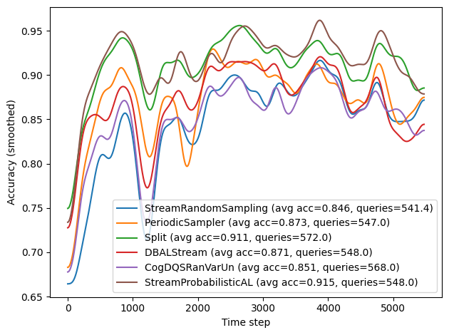
Active Learning Results

The plotting block takes the aggregated data in results and turns it into learning curves for each query strategy. For every entry in results, it first extracts the 2D array of correctness values, where each row corresponds to one repeat and each column to a time step in the stream. It then averages these correctness values across all repeats to obtain a mean accuracy curve over time. This mean curve is optionally smoothed using a Gaussian filter to reduce noise and make trends more visible.

In addition, the code computes the overall average accuracy (as the mean of the mean curve) and the average number of acquired labels across repeats. These summary statistics are encoded directly in the legend label for each query strategy, so each curve is annotated with its mean performance and query usage.

for query_strategy_name, res in results.items():
    correct = res["correct"]
    mean_curve = correct.mean(axis=0)
    smoothed = gaussian_filter1d(mean_curve, 100)

    avg_acc = mean_curve.mean()
    avg_count = res["counts"].mean()

    plt.plot(
        smoothed,
        label=f"{query_strategy_name} (avg acc={avg_acc:.3f}, queries={avg_count:.1f})",
    )

plt.legend()
plt.xlabel("Time step")
plt.ylabel("Accuracy (smoothed)")
plt.tight_layout()